지금 사용하고 있는 opencv 버전의 설치 위치인
D:\opencv 2.4.9\build\python\2.7\x86
에 있는
cv2.pyd 파일을 다음 위치로 복사한다.
C:\Python27\Lib\site-packages
Python IDLE에서
>>import cv2
특별한 함수가 설치되었는지 유무는
>>help(cv2.SIFT())
또는
>>help(cv2)
등으로 체크할 수 있다.
참고
[1] http://imky.egloos.com/2969966
2014년 12월 22일 월요일

2014년 12월 1일 월요일
OpenCV - Color image In/Out
#pragma once
#include <iostream>
#include <opencv/cv.h>
#include <opencv/highgui.h>
using namespace std;
using namespace cv;
// Write grayscale image
void WriteIm(String str, unsigned char* im, const Size& sz)
{
Mat bIm = Mat(sz.height, sz.width, CV_8UC1, im);
imwrite(str, bIm);
}
void main()
{
Mat image = imread("face.jpg");
if (image.empty()) return;
cv::Size sz = image.size();
// hsl channel split
Mat hsl;
cvtColor(image, hsl, CV_RGB2HLS);
Mat hslChannels[3];
split(hsl, hslChannels);
unsigned char *im_l = hslChannels[1].ptr<unsigned char>();
unsigned char *im_h = hslChannels[0].ptr<unsigned char>();
unsigned char *im_s = hslChannels[2].ptr<unsigned char>();
// rgb channel split
Mat rgbChannels[3];
split(image, rgbChannels);
unsigned char *im_r = rgbChannels[0].ptr<unsigned char>();
unsigned char *im_g = rgbChannels[1].ptr<unsigned char>();
unsigned char *im_b = rgbChannels[2].ptr<unsigned char>();
// access image pointer
for(int i=0; i<sz.height; i++)
{
for(int j=0; j<sz.width; j++)
{
im_r[i*sz.width+j] = 255 - im_r[i*sz.width+j];
}
}
// Write image
WriteIm("inv_red.jpg", im_r, sz);
waitKey();
}
#include <iostream>
#include <opencv/cv.h>
#include <opencv/highgui.h>
using namespace std;
using namespace cv;
// Write grayscale image
void WriteIm(String str, unsigned char* im, const Size& sz)
{
Mat bIm = Mat(sz.height, sz.width, CV_8UC1, im);
imwrite(str, bIm);
}
void main()
{
Mat image = imread("face.jpg");
if (image.empty()) return;
cv::Size sz = image.size();
// hsl channel split
Mat hsl;
cvtColor(image, hsl, CV_RGB2HLS);
Mat hslChannels[3];
split(hsl, hslChannels);
unsigned char *im_l = hslChannels[1].ptr<unsigned char>();
unsigned char *im_h = hslChannels[0].ptr<unsigned char>();
unsigned char *im_s = hslChannels[2].ptr<unsigned char>();
// rgb channel split
Mat rgbChannels[3];
split(image, rgbChannels);
unsigned char *im_r = rgbChannels[0].ptr<unsigned char>();
unsigned char *im_g = rgbChannels[1].ptr<unsigned char>();
unsigned char *im_b = rgbChannels[2].ptr<unsigned char>();
// access image pointer
for(int i=0; i<sz.height; i++)
{
for(int j=0; j<sz.width; j++)
{
im_r[i*sz.width+j] = 255 - im_r[i*sz.width+j];
}
}
// Write image
WriteIm("inv_red.jpg", im_r, sz);
waitKey();
}
2014년 11월 30일 일요일
Python에서 sqlite를 이용한 BoVW 구현
# Python에서 sqlite를 이용한 BoVW 구현
# funMV, 2014.12
from numpy import *
import pickle
from pysqlite2 import dbapi2 as sqlite
import sift
import imagesearch
f = open("ukbench/first1000/list.txt",'r') # to access sub-directory
lines = f.readlines() # read all lines through line to line style
f.close()
imlist=[ 'ukbench/first1000/'+line[:-1] for line in lines] # to eliminate last character '\n'
nbr_images=len(imlist)
featlist=[ imlist[i][:-3]+'sift' for i in range(nbr_images)] # filename.sift in each line
# load vocabulary
with open('vocabulary.pkl','rb') as f:
voc = pickle.load(f)
# create db
con = sqlite.connect('test1.db') # 재 실행시, 반드시 test1.db를 지우고 돌려야 함
# 일단, 실행되면 hdd에 test1.db가 저장되기 때문
# create tables
con.execute('create table imlist(filename)')
con.execute('create table imwords(imid,wordid,vocname)')
con.execute('create table imhistograms(imid,histogram,vocname)')
# 다음 4개 명령은 없어도 실행되지만 좀 느려지는 것 같음
con.execute('create index im_idx on imlist(filename)')
con.execute('create index wordid_idx on imwords(wordid)')
con.execute('create index imid_idx on imwords(imid)')
con.execute('create index imidhist_idx on imhistograms(imid)')
con.commit()
# test db
locs, descr = sift.read_features_from_file(featlist[0])
# locs=2276x4, descr=2276x128
# For first image, 2277 features are there and they will be prjected to vw
imwords=voc.project(descr)
#voc.shape[0]=498: # of visual words
#imwords.shape=498의 히스토그램(보팅) 정보
#imwords: voting number of features per each word (histogram). some features among 2278 features
# are voted 7 times to first word, and 6 times for second words of vw, so on.
#array([ 7., 6., 2., 1., 5., 4., 4., 1., 0., 4., 2.,
# 3., 6., 1., 2., 4., 2., 0., 1., 9., 1., 1.,
# 2., 3., 0., 1., 7., 3., 2., 7., 3., 0., 5.,
# 17., 1., 3., 16., 6., 3., 8., 26., 11., 1., 10.,
# 3., 3., 4., 2., 2., 1., 2., 1., 2., 2., ...
nbr_words=imwords.shape[0] # 498
# 위는 test모드이고 여기서부터는 실제 모든 im의 feature들을 db에 삽입
# go through all images, project features on vocabulary and insert
for i in range(nbr_images)[:100]: # [0,1,2,...,98,99]
locs, descr = sift.read_features_from_file(featlist[i])
imname = imlist[i]
imwords=voc.project(descr)
nbr_words=imwords.shape[0]
# (1) 파일 이름을 db에 저장
cur=con.execute("insert into imlist(filename) values ('%s')" %imname)
imid = cur.lastrowid
# (2) 파일 이름 id - 각 word에 대한 voting 횟수 연계 저장
for j in range(nbr_words):
word = imwords[j]
con.execute("insert into imwords(imid,wordid,vocname) values (?,?,?)",
(imid,word,voc.name))
# (3) 파일이름 id와 히스토그램 전체 저장
con.execute("insert into imhistograms(imid,histogram,vocname) values (?,?,?)",
(imid,pickle.dumps(imwords),voc.name))
# 여기서 최종 결과를 저장하고 나가려면 commit를 해 주여야 함.
# con.commit()
# 다시 사용 시
# con=sqlite.connect('test1.db')
#
# Test for saved db
print con.execute('select count (filename) from imlist').fetchone()
# (100,), 100개의 im name이 저장
print con.execute('select * from imlist').fetchone()
# (u'ukbench/first1000/ukbench00000.jpg',)
##################################################
# 여기서 부터 저장된 db를 이용한 test
##################################################
# test할 query인 첫번째 im의 id, 히스토그램을 가져옴
im_id = con.execute("select rowid from imlist where filename='%s'" % imlist[0]).fetchone()
#im_id=(1,)
s = con.execute("select histogram from imhistograms where rowid='%d'" % im_id).fetchone()
h = pickle.loads(str(s[0])) # len(.)=498, histogram for word voting
#Using the index to get candidates
#locs, descr = sift.read_features_from_file(featlist[0])
#imwords=voc.project(descr)
#words=imwords.nonzero()[0] #voting이 하나라도 있는 words의 index
words=h.nonzero()[0]
#vw에 대한 histogram(bin수는 보팅 횟수가 0인 빈을 배제 후 vw의 갯수 만큼)
# words.shape=(455,)=[0,1,2,3,5,....]
# find candidates
candidates = []
for word in words:
# table imword에서 word id로 imid를 추출. 즉, 특정 word를 가진 모든 im의 id를 추출
# 즉, query im의 해당 word를 가지는 db내 모든 im의 id 리스트를 candidates에 저장
im_ids = con.execute("select distinct imid from imwords where wordid=%d"
% word).fetchall()
c = [i[0] for i in im_ids]
candidates += c
# len(candidates) = 1443
# take all unique words and reverse sort on occurrence
tmp = [(w,candidates.count(w)) for w in set(candidates)]
# candidates.count(1)=23, candidates.count(10)=15
# set(candidates)=[1,2,3,4,...,99,100]
# tmp=[(1, 23), (2, 23), (3, 19), (4, 26), (5, 11), (6, 13), (7, 14),
# (8, 11), (9, 28), (10, 15), (11, 14), (12, 30), (13, 10),.....
# (95, 27), (96, 31), (97, 19), (98, 16), (99, 18), (100, 17)]
tmp.sort(cmp=lambda x,y:cmp(x[1],y[1]))
tmp.reverse()
candi=[w[0] for w in tmp] # len(candi)=100
#candi=[43,77,44,42,78,79,...,21,84,83]
#필요한 것은 im의 id이므로 sort후 reverse해줌
matchscores=[]
for imid in candi:
s = con.execute("select histogram from imhistograms where rowid='%d'" % imid).fetchone()
cand_h = pickle.loads(str(s[0])) # histogram for word voting
cand_dist = sqrt( sum( voc.idf*(h-cand_h)**2 ) )
matchscores.append( (cand_dist,imid) )
matchscores.sort()
print matchscores[:10]
#[(0.0, 1), (60.812088499474271, 2), (61.547483004618186, 3), (92.620967753952812, 4),
# (100.59065889285603, 34), (107.76370948763174, 28), (108.27892205906744, 25),
# (109.39719124624605, 9), (110.33866766043165, 10), (110.77231202013482, 20)]
con.commit()
con.close()
# funMV, 2014.12
from numpy import *
import pickle
from pysqlite2 import dbapi2 as sqlite
import sift
import imagesearch
f = open("ukbench/first1000/list.txt",'r') # to access sub-directory
lines = f.readlines() # read all lines through line to line style
f.close()
imlist=[ 'ukbench/first1000/'+line[:-1] for line in lines] # to eliminate last character '\n'
nbr_images=len(imlist)
featlist=[ imlist[i][:-3]+'sift' for i in range(nbr_images)] # filename.sift in each line
# load vocabulary
with open('vocabulary.pkl','rb') as f:
voc = pickle.load(f)
# create db
con = sqlite.connect('test1.db') # 재 실행시, 반드시 test1.db를 지우고 돌려야 함
# 일단, 실행되면 hdd에 test1.db가 저장되기 때문
# create tables
con.execute('create table imlist(filename)')
con.execute('create table imwords(imid,wordid,vocname)')
con.execute('create table imhistograms(imid,histogram,vocname)')
# 다음 4개 명령은 없어도 실행되지만 좀 느려지는 것 같음
con.execute('create index im_idx on imlist(filename)')
con.execute('create index wordid_idx on imwords(wordid)')
con.execute('create index imid_idx on imwords(imid)')
con.execute('create index imidhist_idx on imhistograms(imid)')
con.commit()
# test db
locs, descr = sift.read_features_from_file(featlist[0])
# locs=2276x4, descr=2276x128
# For first image, 2277 features are there and they will be prjected to vw
imwords=voc.project(descr)
#voc.shape[0]=498: # of visual words
#imwords.shape=498의 히스토그램(보팅) 정보
#imwords: voting number of features per each word (histogram). some features among 2278 features
# are voted 7 times to first word, and 6 times for second words of vw, so on.
#array([ 7., 6., 2., 1., 5., 4., 4., 1., 0., 4., 2.,
# 3., 6., 1., 2., 4., 2., 0., 1., 9., 1., 1.,
# 2., 3., 0., 1., 7., 3., 2., 7., 3., 0., 5.,
# 17., 1., 3., 16., 6., 3., 8., 26., 11., 1., 10.,
# 3., 3., 4., 2., 2., 1., 2., 1., 2., 2., ...
nbr_words=imwords.shape[0] # 498
# 위는 test모드이고 여기서부터는 실제 모든 im의 feature들을 db에 삽입
# go through all images, project features on vocabulary and insert
for i in range(nbr_images)[:100]: # [0,1,2,...,98,99]
locs, descr = sift.read_features_from_file(featlist[i])
imname = imlist[i]
imwords=voc.project(descr)
nbr_words=imwords.shape[0]
# (1) 파일 이름을 db에 저장
cur=con.execute("insert into imlist(filename) values ('%s')" %imname)
imid = cur.lastrowid
# (2) 파일 이름 id - 각 word에 대한 voting 횟수 연계 저장
for j in range(nbr_words):
word = imwords[j]
con.execute("insert into imwords(imid,wordid,vocname) values (?,?,?)",
(imid,word,voc.name))
# (3) 파일이름 id와 히스토그램 전체 저장
con.execute("insert into imhistograms(imid,histogram,vocname) values (?,?,?)",
(imid,pickle.dumps(imwords),voc.name))
# 여기서 최종 결과를 저장하고 나가려면 commit를 해 주여야 함.
# con.commit()
# 다시 사용 시
# con=sqlite.connect('test1.db')
#
# Test for saved db
print con.execute('select count (filename) from imlist').fetchone()
# (100,), 100개의 im name이 저장
print con.execute('select * from imlist').fetchone()
# (u'ukbench/first1000/ukbench00000.jpg',)
##################################################
# 여기서 부터 저장된 db를 이용한 test
##################################################
# test할 query인 첫번째 im의 id, 히스토그램을 가져옴
im_id = con.execute("select rowid from imlist where filename='%s'" % imlist[0]).fetchone()
#im_id=(1,)
s = con.execute("select histogram from imhistograms where rowid='%d'" % im_id).fetchone()
h = pickle.loads(str(s[0])) # len(.)=498, histogram for word voting
#Using the index to get candidates
#locs, descr = sift.read_features_from_file(featlist[0])
#imwords=voc.project(descr)
#words=imwords.nonzero()[0] #voting이 하나라도 있는 words의 index
words=h.nonzero()[0]
#vw에 대한 histogram(bin수는 보팅 횟수가 0인 빈을 배제 후 vw의 갯수 만큼)
# words.shape=(455,)=[0,1,2,3,5,....]
# find candidates
candidates = []
for word in words:
# table imword에서 word id로 imid를 추출. 즉, 특정 word를 가진 모든 im의 id를 추출
# 즉, query im의 해당 word를 가지는 db내 모든 im의 id 리스트를 candidates에 저장
im_ids = con.execute("select distinct imid from imwords where wordid=%d"
% word).fetchall()
c = [i[0] for i in im_ids]
candidates += c
# len(candidates) = 1443
# take all unique words and reverse sort on occurrence
tmp = [(w,candidates.count(w)) for w in set(candidates)]
# candidates.count(1)=23, candidates.count(10)=15
# set(candidates)=[1,2,3,4,...,99,100]
# tmp=[(1, 23), (2, 23), (3, 19), (4, 26), (5, 11), (6, 13), (7, 14),
# (8, 11), (9, 28), (10, 15), (11, 14), (12, 30), (13, 10),.....
# (95, 27), (96, 31), (97, 19), (98, 16), (99, 18), (100, 17)]
tmp.sort(cmp=lambda x,y:cmp(x[1],y[1]))
tmp.reverse()
candi=[w[0] for w in tmp] # len(candi)=100
#candi=[43,77,44,42,78,79,...,21,84,83]
#필요한 것은 im의 id이므로 sort후 reverse해줌
matchscores=[]
for imid in candi:
s = con.execute("select histogram from imhistograms where rowid='%d'" % imid).fetchone()
cand_h = pickle.loads(str(s[0])) # histogram for word voting
cand_dist = sqrt( sum( voc.idf*(h-cand_h)**2 ) )
matchscores.append( (cand_dist,imid) )
matchscores.sort()
print matchscores[:10]
#[(0.0, 1), (60.812088499474271, 2), (61.547483004618186, 3), (92.620967753952812, 4),
# (100.59065889285603, 34), (107.76370948763174, 28), (108.27892205906744, 25),
# (109.39719124624605, 9), (110.33866766043165, 10), (110.77231202013482, 20)]
con.commit()
con.close()
Bag of Visual Words

Bag of Words의 요약:

# BoW를 이해하기 위한 Toy example
# BoW algorithm analysis
# 2013/06/28, 2014/12/03 개선
# by funmv
#
from PIL import Image
from pylab import *
import os
from numpy import *
from scipy.cluster.vq import *
import sift
import vocabulary
# 물체의 class는 3개이다 (즉, 0~3/4~7/8~11의 4개씩 동일 물체를 다른 자세에서 찍었음. 아래 그림 참조)
imlist = ['ukbench00000.jpg', 'ukbench00001.jpg', 'ukbench00002.jpg', 'ukbench00003.jpg', 'ukbench00004.jpg', 'ukbench00005.jpg', 'ukbench00006.jpg', 'ukbench00007.jpg', 'ukbench00008.jpg', 'ukbench00009.jpg', 'ukbench00010.jpg', 'ukbench00011.jpg']
nbr_images=len(imlist)
featlist=[ imlist[i][:-3]+'sift' for i in range(nbr_images)]
"""for i in range(nbr_images):
sift.process_image(imlist[i], featlist[i])
"""
descr = []
descr.append(sift.read_features_from_file(featlist[0])[1])
descriptors = descr[0]
# sift.read_features_from_file(featlist[i])[0]:
# list of [pixel coord of each feature point, scale, rotation angle] for i-image
# size: (# of feature point x 4) for i-th image
#
# sift.read_features_from_file(featlist[i])[1]:
# list of [feature values] for i-th image
# size: (# of feature point x 128) for i-th image
for i in arange(1, nbr_images):
descr.append(sift.read_features_from_file(featlist[i])[1])
descriptors = vstack((descriptors, descr[i])) # stack of vector
#len(descr[0]): number of feature points -> 2276
#len(descr[0][1]): size of 1st feature vector -> 128
voc, distortion = kmeans(descriptors[::10,:],3,1) # select one per 10 rows, 3개의 word를 뽑아냄
len(voc) #3, voc = 3x128
len(voc[0]) #3
len(voc[1]) #128
nbr_words = voc.shape[0] #3
# (# of images, bins of histogram(= # of words))
# = (12x3)
imwords=zeros((nbr_images, nbr_words))
print imwords
words, distance = vq(descr[0],voc) # vector quantization
# len(words)->2276
# words: index vector of the cluster that each feature involves
# [1, 2, 1, 0, 1, 2, ...]
#voca = vocabulary.Vocabulary('ukbenchtest')
for i in range(nbr_images): # def project
hist = zeros((nbr_words))
words, distance = vq(descr[i],voc)
# 현재 im에 대해 각 feature가 속하는 word의 index와 이 word까지의 거리가 리턴
# index를 이용하여 해당 word에 보팅하여 histogram을 만듬
for w in words:
hist[w] += 1
imwords[i] = hist
print imwords # degree that each im involve to each cluster
"""
0 1 2 : cluster index (word가 3개이니까 index는 2까지)
[[ 766. 461. 1049.]: 1st image의 histogram의 모양
[ 725. 451. 1020.]: 2nd image의 "
[ 671. 461. 1133.]: ...
[ 1101. 630. 1403.]
[ 260. 317. 409.]
[ 267. 308. 370.]
[ 283. 394. 476.]
[ 239. 331. 410.]
[ 1105. 468. 1317.]
[ 116. 191. 390.]
[ 122. 251. 439.]
[ 1183. 597. 1475.]]: 12번째 im의 histogram모양
12번째 이미지의 모든 특징 중에서 word 0에 속하는 것은 1183개, 1번 597개, 2번 1475개이다. 3경우 합하면 특징의 개수이다. 따라서 test영상의 특징에 대한 histogram을 그리고 위 12개 중에서 hist모양이 비슷한 것을 찾으면 그것이 해당 영상이다.
"""


다음의 코드에서 voc의 내용을 알 수 있음.

2014년 8월 17일 일요일
Blog Visited
[Unit test]
C++ 프로젝트에 단위 테스트 도입하기
http://www.slideshare.net/mobile/zone0000/c-7522148
stinkfist : 구글테스트 시작하기
http://stinkfist.egloos.com/m/2262578
Rebooting Reiot
http://reiot.com/2008/07/04/google-test/
googletest 환경 구축 :: moltak
http://moltak.tistory.com/m/post/295
[LSH]
다음 블로그 NLP: http://blog.daum.net/hazzling?bz=blog
LSH(locality sensitive hashing)
GibHub로 이사: http://dsindex.github.io/
[DreamPark]
Windows Embeded 8.1 Industry Pro 리뷰:
http://ccami.tistory.com/92
MS dreampark에서 대학계정 무료 배포
[SWIG]
SWIG Tutorial
http://ppiazi.tistory.com/m/post/entry/SWIG-Tutorial#
C/C++ Wrapping에 의한 Tcl, Perl, Python, Java, C# 함수 제공
[SQLite]
SQLite 와 C++ 연동방법 :: 인생의무한루프
http://mins79.tistory.com/entry/SQLite-%EC%99%80-C-%EC%97%B0%EB%8F%99%EB%B0%A9%EB%B2%95
수까락의 프로그래밍 이야기 : SQLite - 튜토리얼 with CppSQLite
http://sweeper.egloos.com/m/3053076
CppSQLite - C++ Wrapper for SQLite - CodeProject
[Consumer Camera]
[usb3 Camera]
Buy e-con's Camera Boards | Camera Modules | Computer on Modules | Reference designs
http://www.e-consystems.com/webstore.asp
[Graphics Models]
Classical Probabilistic Models and Conditional Random Fields
http://www.scai.fraunhofer.de/fileadmin/images/bio/data_mining/paper/crf_klinger_tomanek.pdf
Machine Learning: Generative and Discriminative Models
http://www.cedar.buffalo.edu/~srihari/CSE574/Discriminative-Generative.pdf
[MCMC]
Sampling and MCMC (intractable integral)
http://arongdari.tistory.com/m/post/62#
Sampling and Markov Chain Monte Carlo
http://www.stat.cmu.edu/~larry/=sml2008/lect2.pdf
Toy code
http://www.ece.sunysb.edu/~zyweng/MCMCexample.html
Monte Carlo Methods
http://www.cs.cmu.edu/~ggordon/MCMC/
Impacted paper
http://citeseerx.ist.psu.edu/viewdoc/download?doi=10.1.1.13.7133&rep=rep1&type=pdf
Sampling & MCMC
http://arongdari.tistory.com/m/post/entry/Sampling-MCMC#
[L1-Regularized Min]
Parallel Coordinate Descent for L1-Regularized Loss Minimization
http://www.select.cs.cmu.edu/publications/paperdir/icml2011-bradley-kyrola-bickson-guestrin.pdf
[GoPro Hero4 Livestream]
http://www.reddit.com/r/gopro/comments/2md8hm/how_to_livestream_from_a_gopro_hero4/
OpenCV in C++
https://gist.github.com/KonradIT/8554673
#include <opencv2/opencv.hpp>
int main()
{
cv::VideoCapture cap( "http://10.5.5.9:8080/live/amba.m3u8" );
cv::namedWindow( "GoPro" );
cv::Mat frame;
do {
cap >> frame;
cv::imshow( "GoPro", frame );
} while ( cv::waitKey( 30 ) < 0 );
return 0;
}
C++ 프로젝트에 단위 테스트 도입하기
http://www.slideshare.net/mobile/zone0000/c-7522148
stinkfist : 구글테스트 시작하기
http://stinkfist.egloos.com/m/2262578
Rebooting Reiot
http://reiot.com/2008/07/04/google-test/
googletest 환경 구축 :: moltak
http://moltak.tistory.com/m/post/295
[LSH]
다음 블로그 NLP: http://blog.daum.net/hazzling?bz=blog
LSH(locality sensitive hashing)
GibHub로 이사: http://dsindex.github.io/
[DreamPark]
Windows Embeded 8.1 Industry Pro 리뷰:
http://ccami.tistory.com/92
MS dreampark에서 대학계정 무료 배포
[SWIG]
SWIG Tutorial
http://ppiazi.tistory.com/m/post/entry/SWIG-Tutorial#
C/C++ Wrapping에 의한 Tcl, Perl, Python, Java, C# 함수 제공
[SQLite]
SQLite 와 C++ 연동방법 :: 인생의무한루프
http://mins79.tistory.com/entry/SQLite-%EC%99%80-C-%EC%97%B0%EB%8F%99%EB%B0%A9%EB%B2%95
수까락의 프로그래밍 이야기 : SQLite - 튜토리얼 with CppSQLite
http://sweeper.egloos.com/m/3053076
CppSQLite - C++ Wrapper for SQLite - CodeProject
MFC + SQLite3 연동 :: 개발환경을 만들자
[運]과 함께하는 세상 : SQLite 와 C++ 연동방법
SQLite 쿼리 간단 사용법 매뉴얼 기본 동작 상세 설명 :: 포쿠테
[Matlab]
MATLAB 때려잡기 - 01강 - Modern Control Theory 때려잡기 - What is Control Theory?
[Consumer Camera]
범용 카메라를 이용한 이미지 처리: Nikon Imaging | SDK Download
[usb3 Camera]
http://www.e-consystems.com/webstore.asp
[Graphics Models]
Classical Probabilistic Models and Conditional Random Fields
http://www.scai.fraunhofer.de/fileadmin/images/bio/data_mining/paper/crf_klinger_tomanek.pdf
Machine Learning: Generative and Discriminative Models
http://www.cedar.buffalo.edu/~srihari/CSE574/Discriminative-Generative.pdf
discriminative vs. generative, classification vs. categorization
[MCMC]
Sampling and MCMC (intractable integral)
http://arongdari.tistory.com/m/post/62#
Sampling and Markov Chain Monte Carlo
http://www.stat.cmu.edu/~larry/=sml2008/lect2.pdf
Toy code
http://www.ece.sunysb.edu/~zyweng/MCMCexample.html
Monte Carlo Methods
http://www.cs.cmu.edu/~ggordon/MCMC/
Impacted paper
http://citeseerx.ist.psu.edu/viewdoc/download?doi=10.1.1.13.7133&rep=rep1&type=pdf
Sampling & MCMC
http://arongdari.tistory.com/m/post/entry/Sampling-MCMC#
[L1-Regularized Min]
Parallel Coordinate Descent for L1-Regularized Loss Minimization
http://www.select.cs.cmu.edu/publications/paperdir/icml2011-bradley-kyrola-bickson-guestrin.pdf
[GoPro Hero4 Livestream]
The new HERO4 Black and Silver edition cameras use a different, more powerful chip (ambarella A9). The traditional URL for HERO2/HERO3/HERO3+ http://10.5.5.9:8080/live/amba.m3u8 does not work for the new HERO4 camera.
Here is how to get the live stream:
- Open this URL: http://10.5.5.9/gp/gpExec?p1=gpStreamA9&c1=restart
- In VLC/FFplay/other open the udp port: udp://:8554
- Make sure the media player is configured as mpeg streaming.
http://www.reddit.com/r/gopro/comments/2md8hm/how_to_livestream_from_a_gopro_hero4/
OpenCV in C++
https://gist.github.com/KonradIT/8554673
#include <opencv2/opencv.hpp>
int main()
{
cv::VideoCapture cap( "http://10.5.5.9:8080/live/amba.m3u8" );
cv::namedWindow( "GoPro" );
cv::Mat frame;
do {
cap >> frame;
cv::imshow( "GoPro", frame );
} while ( cv::waitKey( 30 ) < 0 );
return 0;
}
2014년 8월 12일 화요일
Path planning of mobile robot
작성 중...

$V(t)$와 $\omega(t)$는 control input.

로봇의 시작 점과 목표 점이 주어진다고 할 때,
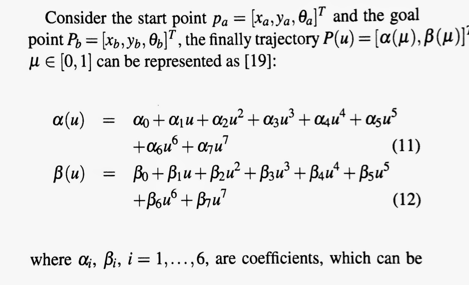
Path는 $P(u)$에 의해 정의된다. 파라메터인 $u$는 0에서 1까지 변하는 값으로 0은 로봇의 시작 점, 1은 목표 점을 가리킨다.
이 수식은 아주 많은 파라메터들로 구성되는데 이 값들을 바꾸면 다양한 형태의 path가 생성된다 [1].

만일 장애물을 회피하여 목표 점까지 이동한다 가정하자. 경로는 시작 위치에서 장애물을 피하고 목표 위치로 부드럽게 수렴하는 경로를 얻는 것이 필요하다.
여러 파라메터 중에서 2개의 파라메터를 고려하면,
$Path=f(\eta_3, \theta_a)$
이고 path는 다양한 파라메터 중에서 두 변수가 중요하게 작용하므로 이들의 함수이다.
현재 로봇이 가진 각도를 기준으로 전방 180도로 정의하면,
$\theta_a$를 0~180에서 10도씩 나누고, 각 $\theta$에 대해 10개의 $\eta$를 정의한다.
그러면 위 그림의 상부와 같은 경로들이 나온다.
즉, 10도씩 나누어 19개의 set가 있고, 각 set 내에는 ($\eta$의 변화에 따라) 10개의 path가 존재한다.
이렇게 정의한 여러 path 중에서 최적인 하나를 선정하는 것이 필요하다.
로봇은 자체 회전이 가능하여 어떤 출발 각도를 가지고도 출발할 수 있다.
이동 경로 길이가 짧으면서 장애물 충돌 없이 목표에 도달하는 것이 필요하다.
예를 들면 출발 각이 목표 각과 비슷하면 경로 길이는 짧아 진다.
경로를 결정하였으면 로봇이 경로를 따라 잘 이동하도록 제어하는 것이 필요하다.

current 위치에서 destination으로 위치와 자세를 바꾸기 위해서 오차를 위 행렬 식처럼 정의한다.

Lyapunov함수를 이용하여 비용함수 $V$를 정의한다. 식을 보면 $x_e, y_e, \theta_e$가 모두 0으로 가면 $V$도 0으로 수렴한다.
References
[1] Lyapunov Theory
Online boosting

초기에 지정된 영역을 5개 부분으로 나누어 (+1/-1)로 학습.
물체 추적 시에는 물체 크기의 window를 sliding시켜 ROI 내부를 검색.
현재 위치에 대해 window 내부의 특징을 classifier로 평가하고 confidence 계산.
ROI 내부의 confidence map를 저장하고, map에 대해 integral image를 적용시켜 최대 confidence 영역을 찾아 냄.
최대 영역이 새로운 물체의 위치(+)가 되고, 이 물체의 배경(-)과 함께 다시 학습(update).
피드 구독하기:
글 (Atom)